Partial Derivatives and Plane Tangents 14.3, 14.4

The following notebook will take the user through five points, showing examples of how to use Python to graph functions of two variables and communicate ideas. It will also familarize the reader with some basic LaTeX syntax.

1. How to plot 2D plots and 3D surfaces + curves in Python with numpy and matplotlib

2. Parametric derivatives, visually

3. Partial derivatives and Tangent Planes

1. Basic Plots in 2D and 3D using matplotlib

Basic Functions in matplotlib for 2D plots

Basic Functions for Plotting 3D Plots

We will plot the following two types of curves

$$Functions \ of \ two \ variables: g(x,y)$$ $$ g(x): \Re ^2 \rightarrow \Re $$ $$Parametric \ Plots: \ r(t) = \ <xt, yt, zt>$$ $$ r(t): \Re ^3 $$

But what does drawing parametric curves look like? We can loop through the array.

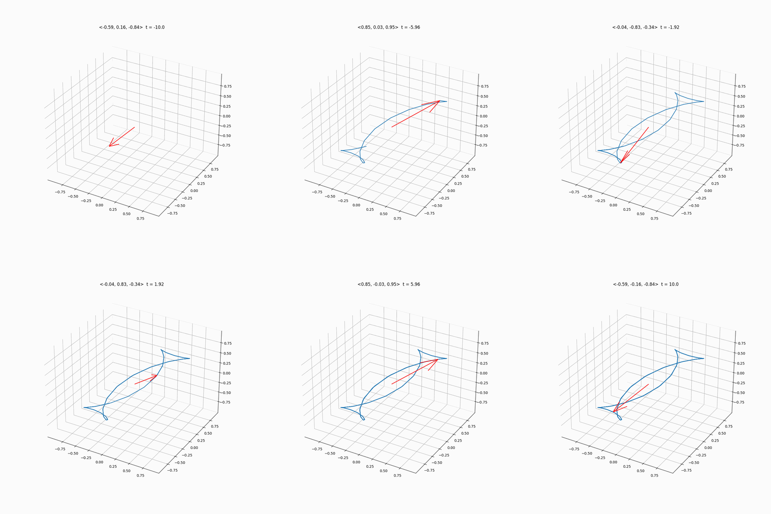
2. Parametric Derivatives

We will use a different parametric equation from the one above. $$ r(t) = <t^2 + 2t, t^2 + t, t + 3> $$ $$ r'(t) = <2t + 2, \ 2t + 1, \ 1> $$ We will find the derivative at $ t = -2 $ through the limit definition of the derivative. $$ \lim_{h \to -2} \frac {r(-2 + h) - r(-2)}{h}

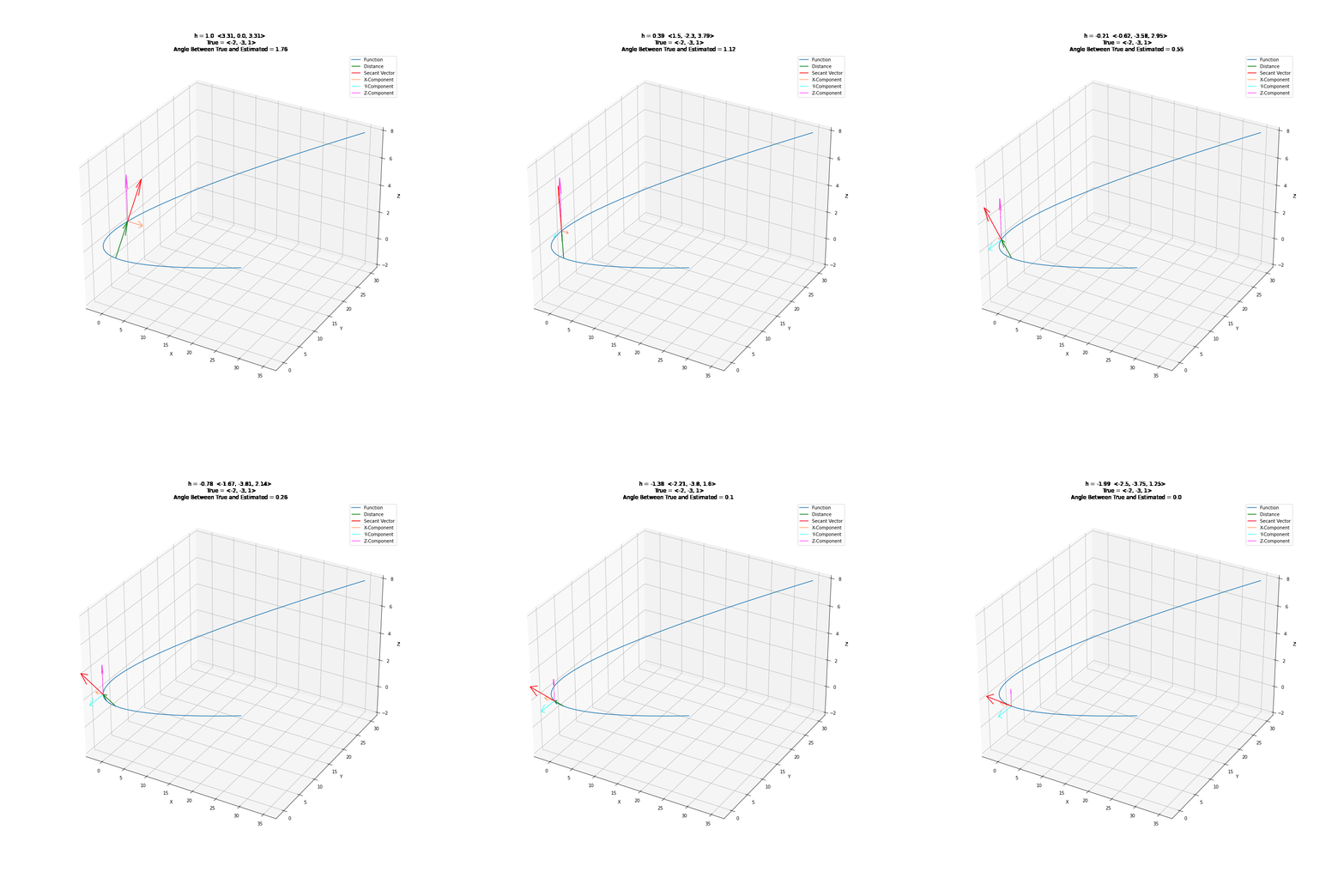
3. Partial Derivatives

To show partial derivatives of functions of two variables, we will first see the trace of surfaces, a technique we can use to draw them by hand. Then we will show the idea of partial derivatives and what they might mean graphically. We will use the curves below as examples.

### Our curves of interest. $$ g(x,y) = 4 - (x^2 + y^2)$$ $$ s(x,y) = sin(x) + sin(y)$$ $$ h(x,y) = x^2 - y^2 $$ $$ r(x,y) = y^2 - x^3 + x $$ We can find the trace of these curves by keeping one of the variables constant, slowly moving it.

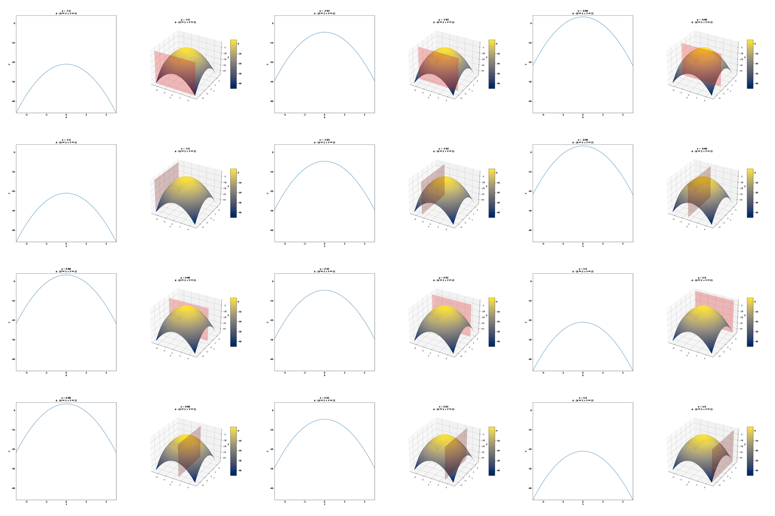
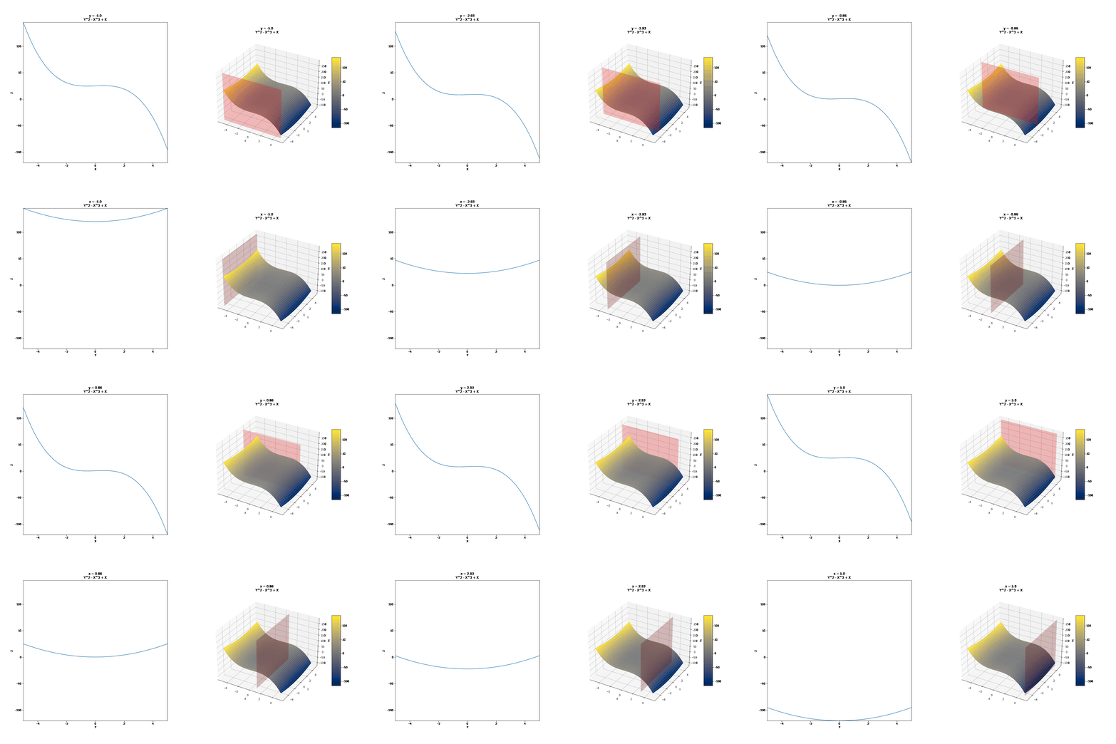
For the changing values of Y, we have different values of Z and X. We can draw a few of these curves and connect them to draw 3D surfaces by hand. For example, we can take y = -4, y = -2, y = 0, y = 2, y = 4, and connect these in a parabolic manner after keeping x constant. It might further help to realize that these are this is where the surface intersects 2D planes. Visualized below are some other surfaces.

Contour or Level Curves (Traces with z = k, k = constant)

Contour curves are a little more interesting to look at.

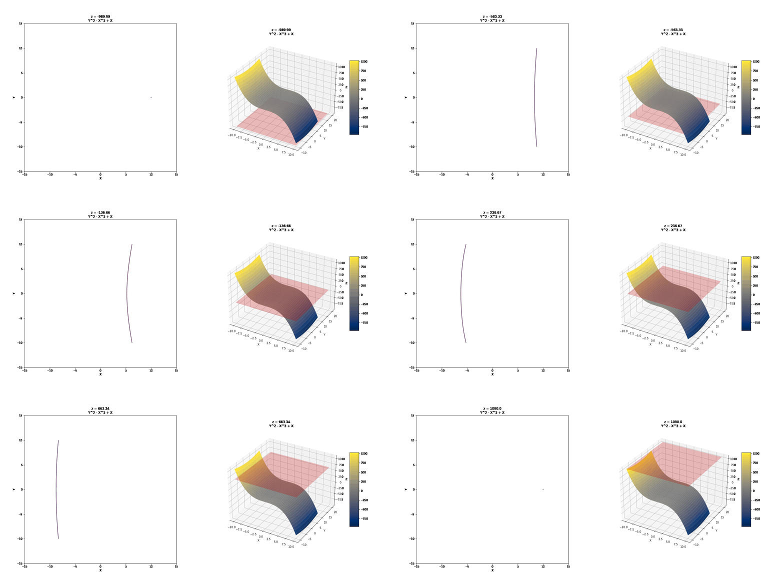
Note the real contour graph below, the usual way it would be drawn

<matplotlib.contour.QuadContourSet at 0x7faf1c6541c0>

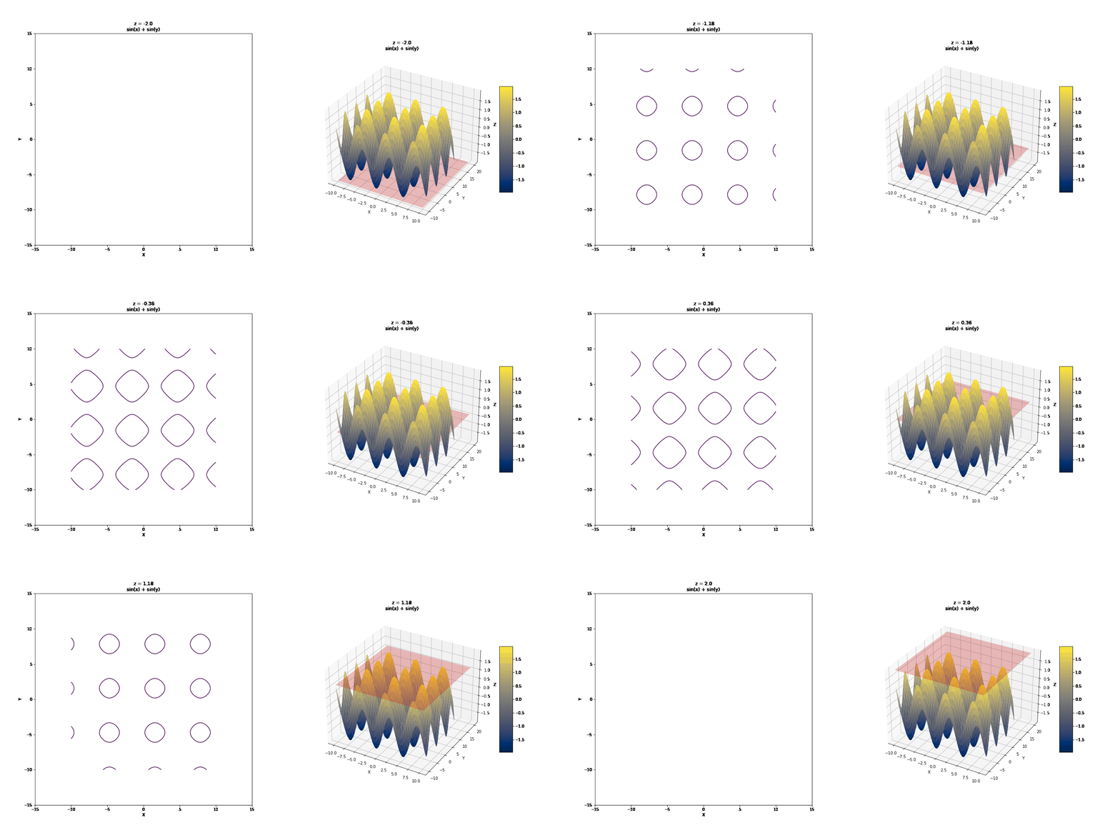
<matplotlib.contour.QuadContourSet at 0x7faee9ed9550>

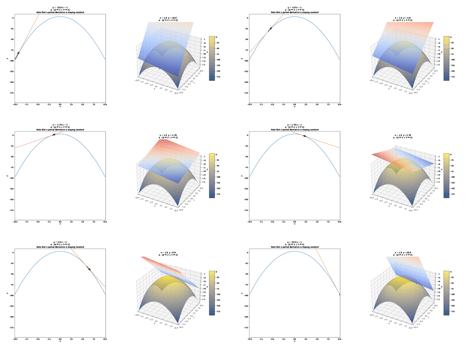
Contour Graphs were a quick aside. We can use the trace with the xz and yz planes to help us understand partial derivatives. Represents the rate of change when one variable is kept fixed.

$$ g(x,y) = 4 - (X^2 + Y^2) $$ $$ \frac{\partial z}{\partial x} = -2x $$ $$ \frac{\partial z}{\partial y} = -2y $$ $$ show \ g'(1,k): $$